Models¶

The models are dictionaries with the properties of a machine or a calculation.

Machine¶

Machines have a set of basic parameters, a stator, a magnet and a winding:

Parameter	Description	Unit
name	Name of machine
lfe	Lenght of iron	m
poles	Number of poles
outer_diam	Outer diameter (yoke side)	m
bore_diam	Bore diameter (airgap side)	m
inner_diam	Inner diameter (yoke)	m
airgap	airgap width	m
external_rotor	True, False	False
ffactor	processing factor for iron losses
dxffile	(see Model Creation with DXF)

Stator¶

Stators have basic parameters and slots:

Parameter	Description	Default
num_slots	Number of Slots Q
num_slots_gen	Number of Slots in Model	mQ/gcd(Q, 2pm)
rlength	Relative iron length	1.0
mcvkey_yoke	Name of lamination material	dummy
mcvkey_teeth	Name of lamination material	dummy
nodedist	Factor for node distance	1.0

Note

if no value for num_slots_gen is given its value is calculated from the the number of slots Q and pole pairs p. (version added 0.0.16)

Stator Slots¶

Name	Parameter
stator1	slot_rf1, tip_rh1, tip_rh2, tooth_width, slot_width
stator2	slot_t1, slot_t2, slot_t3, slot_depth, slot_width, corner_width
statorRotor3	slot_height, slot_h1, slot_h2, slot_width, slot_r1, slot_r2, wedge_width1, wedge_width2, middle_line, tooth_width, slot_top_sh
stator4	slot_height, slot_h1, slot_h2, slot_h3, slot_h4, slot_width, slot_r1, wedge_width1, wedge_width2, wedge_width3
statorBG	yoke_diam_ins slot_h1, slot_h3, slot_width, slot_r1, slot_r2, middle_line, tooth_width, tip_rad, slottooth
<filename>	(see User defined Stator Slots with FSL)
dxffile	(see User defined Slots with DXF)

Note

All units are metric units.

User defined Stator Slots with FSL¶

If a FSL file that includes the definition of stator geometry exists and is readable it can be used for the model creation.

Example with file mystator.fsl:

machine = dict(
    name="Motor",
    ...
    stator=dict(
        mcvkey_yoke='dummy',
        mcvkey_shaft="dummy",
        mystator=dict()
    ),
    ...

User defined Slots with DXF¶

If a DXF file that defines the stator geometry exists and is readable it can be used to create the FSL of the model. All DXF conversion parameters are supported.

Example:

machine = dict(
    name="Motor",
    ...
    stator=dict(
        mcvkey_yoke='dummy',
        dxffile=dict(
            name="mystator.dxf",
            position='out',
            split=True
        )
    ),
    ...

Parameters	Description	Default
position	‘in’ or ‘out’
split	splits intersecting lines at their intersection-points	False
plot	creates the plot of the integrated object	False

– Note:: The split option is required only if intersecting lines have no common point.

Windings¶

Name	Parameter	Default
num_phases	number of phases (m)
num_wires	number of wires per slot
coil_span	coil span
num_layers	number of layers
cufilfact	Fill factor of copper	0.45
culength	rel length of conductor	1.4
cuconduc	conductivity (S/m)	56e6
slot_indul	insulation thickness in slot	0.0

Windings may contain a leakage dict: leak_dist_wind, leak_evol_wind, leak_tooth_wind (version added 0.9.9)

leak_dist_wind

Name

Parameter

Unit

perimrad

Radius of perimeter

m

vbendrad

Bending radius vertical

m

endheight

End winding height

m

m.wiredia

Wire diameter

m

leak_evol_wind

Name	Parameter	Unit
evol1rad	Top radius of first evolvent	m
evol2rad	Top radius of second evolvent	m
botlevel	Level at bottom of evolvents	m
toplevel	Level at top of evolvents	m
evolbend	Bending radius	m
endheight	End winding height	m
m.wiredia	Wire diameter	m

leak_tooth_wind

Name	Parameter	Unit
bendrad	Bending radius vertical	m
endheight	End winding height	m
m.wiredia	Wire diameter	m

Example:

windings=dict(
    num_phases=3,
    num_wires=100,
    coil_span=3.0,
    num_layers=1,
    leak_dist_wind=dict(
        perimrad=67.1e-3, # Radius of perimeter [m]
        vbendrad=5e-3,    # Bending radius vertical [m]
        endheight=20e-3,  # End winding height [m]
        wiredia=1e-3)     # Wire diameter [m]
)

Magnet¶

Magnets have basic parameters and slots:

Parameter	Description	Default
mcvkey_yoke	Name of lamination material	dummy
mcvkey_shaft	Name of shaft material	dummy
material	Name of magnet material
nodedist	Factor for node distance	1.0

Note

the mcvkey parameters either reference a filename without extension (Example ‘M330-50A’) which must be found in the directory defined by the parameter magnetizingCurves of the Femag constructor or the name of an entry in the magnetizingCurve object.
the material parameter references a name of the ‘Magnet Material’_ list.

Rotor Slots¶

Name	Parameter
magnetSector	magn_num, magn_width_pct, magn_height, magn_shape, bridge_height, magn_type, condshaft_r, magn_ori, magn_rfe, bridge_width, magn_len
magnetIron	magn_height, magn_width, gap_ma_iron, air_triangle, iron_height, magn_rem, condshaft_r, magn_ori, bridge_height, bridge_width, iron_shape
magnetIron2	magn_height, magn_width, gap_ma_iron, air_triangle, iron_height, magn_rem, condshaft_r, gap_ma_right, gap_ma_left, magn_ori, iron_shape
magnetIron3	magn_height, iron_bfe, gap_ma_iron, air_triangle, iron_height, gap_ma_right, gap_ma_left, condshaft_r, magn_num, magn_ori, iron_shape
magnetIron4	magn_height, magn_width, gap_ma_iron, iron_shape, air_space_h, iron_bfe, magn_di_ra, corner_r, air_sp_ori, magn_ori, magn_num
magnetIron5	magn_height, magn_width, gap_ma_iron, iron_bfe, air_space_h, corner_r, air_sp_ori, magn_num, iron_shape, air_space_b, magn_di_ra
magnetIronV	magn_height, magn_width, magn_angle, magn_num, iron_hs, iron_height, iron_shape, air_triangle, gap_ma_iron, magn_rem, condshaft_r
magnetFC2	yoke_height, iron_h1, iron_h2, iron_b, magn_width, magn_height, iron_bfe, iron_bfo, iron_shape, iron_hp, magn_num
<filename>	see User defined Magnet Slots with FSL
dxffile	see User defined Slots with DXF

Example:

machine = dict(
   name="PM 130 L4",
   lfe=0.1,
   poles=4,
   outer_diam=0.13,
   bore_diam=0.07,
   inner_diam=0.015,
   airgap=0.001,

   stator=dict(
       num_slots=12,
       num_slots_gen=3,
       mcvkey_yoke="dummy",
       rlength=1.0,
       stator1=dict(
           slot_rf1=0.057,
           tip_rh1=0.037,
           tip_rh2=0.037,
           tooth_width=0.009,
           slot_width=0.003)
       ),

   magnet=dict(
       mcvkey_shaft="dummy",
       mcvkey_yoke="dummy",
       magnetSector=dict (
           magn_num=1,
           magn_width_pct=0.8,
           magn_height=0.004,
           magn_shape=0.0,
           bridge_height=0.0,
           magn_type=1,
           condshaft_r=0.02,
           magn_ori=2,
           magn_rfe=0.0,
           bridge_width=0.0,
           magn_len=1.0 )
       ),

    windings=dict(
         num_phases=3,
         num_wires=100,
         coil_span=3.0,
         num_layers=1)
)

User defined Magnet Slots with FSL¶

Example

If a FSL file that creates the magnet geometry exists and is readable it can be used for the model creation as an empty dict:

machine = dict(
    name="Motor",
    ...
    magnet=dict(
        mcvkey_yoke='dummy',
        mcvkey_shaft="dummy",
        myrotor=dict()
    ),
    ...

User defined Slots with DXF¶

If a DXF file that defines the magnet geometry exists and is readable it can be used to create the FSL for the model.

Example:

machine = dict(
    name="Motor",
    ...
    magnet=dict(
        mcvkey_yoke='dummy',
        mcvkey_shaft="dummy",
        dxffile=dict(
            name='mymagnet.dxf',
            position='in',
            split=True
        )
    ),
    ...

Parameters	Description	Default
position	‘in’ or ‘out’
split	splits intersecting lines at their intersection points	False
plot	creates the plot of the integrated object	False

– Note:: The split option is required only if intersecting lines have no common point.

Magnetizing Curve¶

The MagnetizingCurve is a container of magnetizing curves (eg. lamination or PM material) that can be referenced by the model mcvkey attributes. It can either point to a directory of MC/MCV-File or hold a list of magnet curves which are identified by name.

Each magnetizing curve is described by the following properties

Attribute	Description	Unit	Default
name	Identifier of this curve
ctype	Type of curve		1
desc	Description
curve	List of dictionaries with bi (list of induction values) hi (List of field strength values) and angle which can be missing in case of 1 curve	T, A/m, deg
ch	hysteresis loss factor		0
cw	eddy current loss factor		0
ch_freq	hysteresis exponent		0
cw_freq	eddy-current exponent		0
b_coeff	induction loss exponent		0
Bo	reference induction	T	1.5
fo	reference frequency	Hz	50
fillfac	iron fill factor		1
bsat	saturation induction	T	2.15
rho	specific weight	kg/dm3	7.65

The loss factors and exponents are used in the Jordan loss calculation formula:

(cw*(f/fo)**cw_freq + ch*(f/fo)**ch_freq)*(B/Bo)**b_coeff

The Reader object which is included in the mcv module can be used to read MCV/MC files.

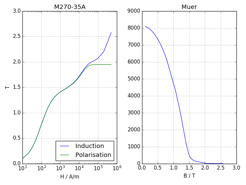
Permeability and polarisation calculation example:

MUE0 = 4e-7*math.pi

mcv = femagtools.mcv.Reader()
mcv.readMcv('magnetcurves/M270-35A.MCV')
r = mcv.get_results()

bh = [(bi, hi)
      for bi, hi in zip(r['curve'][0]['bi'],
                        r['curve'][0]['hi']) if bi > 0 and hi > 0]

ji = [b-MUE0*h for b, h in bh]
muer = [bx/hx/MUE0 for bx, hx in bh]

Using a magnetizingcurve to write a mcv file:

mcvData = dict(curve=[ dict(
   bi=[0.0, 0.09, 0.179, 0.267, 0.358,
       0.45, 0.543, 0.6334, 0.727,
       0.819, 0.9142, 1.0142, 1.102,
       1.196, 1.314, 1.3845, 1.433,
       1.576, 1.677, 1.745, 1.787,
       1.81, 1.825, 1.836],

    hi=[0.0, 22.16, 31.07, 37.25, 43.174,
        49.54, 56.96, 66.11, 78.291,
        95, 120.64, 164.6, 259.36,
        565.86, 1650.26, 3631.12, 5000, 10000,
        15000, 20000, 25000, 30000, 35000, 40000]
    )],
    name='m270-35a',
    desc=u"Demo Steel",
    ch=4.0,
    cw_freq=2.0,
    cw=1.68)

 mcv = femagtools.mcv.MagnetizingCurve(mcvData)

 mcv.writefile('m270-35a')

Note

if the curve data is used in a stator or magnet slot model there is no need to create the file explicitly. Femagtools will take care of that during the model creation.

Magnet Material¶

list of dict objects each having a unique name (or id) and a set of parameters that describe the magnet properties.

Parameter	Description	Default	Unit
name	Name of magnet material
mcvkey	name of nonlinear B(H) curve
orient	Magnetizing orientation	cartiso
rlen	Relative length	1.0
remanenc	Remanence Induction Br		T
relperm	Relative Permeability
spmaweight	Specific Mass	7500	kg/m³
temcoefbr	Temperature Coefficient of Br	-0.001	1/K
temcoefhc	Temperature Coefficient of Hc	-0.001	A/m/K
magntemp	Magnet Temperature	20	°C
magncond	Electr. Conductivity	625000	S/m
magnwidth	Magnet width	0.0	m
magnlength	Magnet length in z direction	0.0	m

Note

name must be unique within list. It may be used as reference in the magnet model of the machine.

Example:
```
magnets = [dict(name='MX-333', remanenc=1.2, relperm=1.05)]
```
mcvkey is used for material that have a non-linear BH curve.
the key orient describes the field orientation (mcartiso, mpoliso, martaniso, mpolaniso)

rlen defines the relative length

Example:

magnets=[dict(name='BH53M', mcvkey='BH53M',
              orient='mcartiso', rlen=1.0)]

The mcvkey can either reference a file or an entry in the magnetizing curve dict.

User Specified Magnet Geometries¶

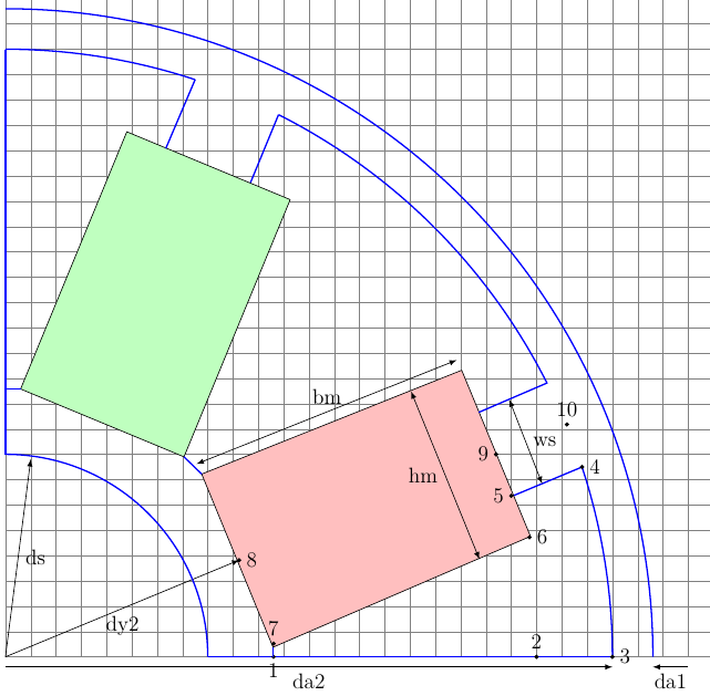
Magnet geometries not covered by the built in models can be specified by fsl code. Here is a example:

Example of a user specified geometry (created with TikZ)¶

The steps are:

Create a diagram of the geometry and decide about the parameters to be used.
Create a fsl mako template file with the chosen parameters as placeholders using the Mako syntax with ${}.
Include this filename in the magnet model within the section using the basename of the mako file and set the parameter values.

The following values are defined globally and can be referenced in the template:

Name	Description	Unit
mcvkey_yoke	lamination material of yoke
mcvkey_shaft	material of shaft
m.remanenc	Remanence Induction	T
m.relperm	Rel. Permeability of PM
m.num_poles	Number of poles
m.npols_gen	Number of poles in model
agndst	Node distance in airgap	m
dy1	Diameter of stator yoke	m
da1	Diameter of stator bore	m
da2	Diameter of rotor	m
dy2	Diameter of rotor yoke	m

Example FSL Template file ‘’spoke.mako’’ using 4 parameters:

-- Model parameters

ds = ${model['shaft_diam']}*1e3
hm = ${model['magn_height']}*1e3
bm = ${model['magn_width']}*1e3
ws = ${model['slot_width']}*1e3

-- calculate slot height and pole pitch
hs = (da2-dy2)/2 - bm
taup = math.pi/m.num_poles

x = {}
y = {}

-- characteristic points of model

ar = math.sqrt(dy2^2+hm^2)/2
x[1] = ar*math.cos(taup - math.atan2(hm/2, dy2/2))
y[1] = 0
x[2],y[2] = pr2c(dy2/2+bm, 0)
x[3],y[3] = pr2c(da2/2, 0)
x[4],y[4] = pr2c(da2/2, taup - math.atan2(ws/2,(da2/2)))
x[5],y[5] = pr2c(da2/2-hs, taup - math.atan2(ws/2,(da2/2 - hs)))
x[6],y[6] = pr2c(da2/2-hs, taup - math.atan2(hm/2, da2/2-hs))
x[7],y[7] = pr2c(ar, taup - math.atan2(hm/2, dy2/2))
x[8],y[8] = pr2c(dy2/2, taup)
x[9],y[9] = pr2c(da2/2 - hs, taup)
x[10],y[10] = pr2c(da2/2, taup)

Magnet definition in Python file with included mako file (eg in this case ‘’spoke’’) and the parameter definition:

..
magnet=dict(
    mcvkey_yoke="dummy",
    spoke=dict(
        magn_height=0.008,
        shaft_diam=0.01,
        slot_width=0.004,
        magn_width=0.024
    )
 ..

The resulting model:

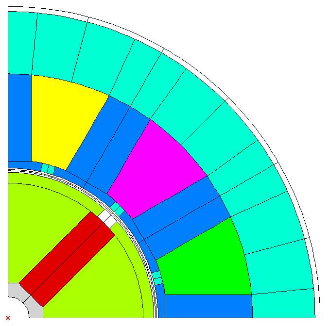
Note

Starting with Release 0.4.4 the syntax has changed but backward compatibility is fully supported.

the complete example can be found in stator1-spoke.py and spokefml.mako in the example directory on github.

FE-Simulation¶

Cogging (cogg_calc)

Parameter	Description	Default	Unit
speed	Speed		1/s
skew_angle	Skewing angle	0	deg
num_skew_steps	Number of skew steps	0
magn_temp	Magnet Temperature		°C
num_move_steps	Number of move steps
num_par_wdgs	Number of parallel windings	1
eval_force	Evaluate force	0
period_frac	Rotate Fraction of Period	1
vtu_movie	Create VTU files	False

Example:

operatingConditions = dict(
  calculationMode="cogg_fast",
  magn_temp=60.0,
  num_move_steps=49,
  speed=50.0)

PM/Rel Machine Simulation (pm_sym_fast)

Parameter	Description	Default	Unit
speed	Speed		1/s
skew_angle	Skewing angle	0	deg
num_skew_steps	Number of skew steps	0
magn_temp	Magnet Temperature		°C
wind_temp	Winding Temperature	20	°C
num_move_steps	Number of move steps	49
num_par_wdgs	Number of parallel windings	1
eval_force	Evaluate force	0
explicit_mode	Activates/deactivates step adjustments	0
current	Phase current		A (RMS)
angl_i_up	Angle I vs. Up	0	deg
optim_i_up	Optimize Current	0
phi_start	Start angle of rotation	0	deg
range_phi	Rotation angle	360/p	deg
explicit_mode	Deactivate rotation correction	0
plots	Create plots	[]
airgap_induc	calculate airgap induction	False
period_frac	Rotate Fraction of Period	1
vtu_movie	Create VTU files	False

Note

plots is a list of field_lines or color_gradation plots to be created after the calculation. Possible values ‘field-lines’, ‘Babs’, ‘Br’, ‘Bx’, ‘By’, ‘Br’, ‘Bt’, ‘Habs’, ‘Hx’, ‘Hy’, ‘Hr’, ‘Ht’ ‘demag’, ‘ecurr’, ‘ecloss’, ‘relperm’, ‘Wm’, ‘Bdev’, ‘Vpot’. (See http://script.profemag.ch/ColorGrad.html) added in version 0.0.16. The value types can be simple strings or list with name and min/max range.

Example:

operatingConditions = dict(
  calculationMode="pm_sym_fast",
  wind_temp=60.0,
  magn_temp=60.0,
  current=50.0,
  speed=50.0,
  plots=['field_lines', ['Babs', 0.0, 2.5]])

Note

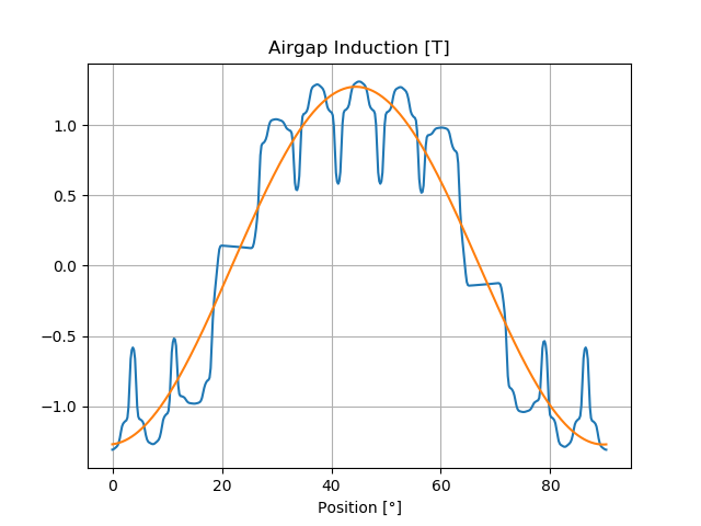
If airgap_induc is True the induction in the airgap is calculated after the simulation returns. The values can be read with the method read_airgap_induc() of call Femag.

Parameter	Description	Unit
Baml	Amplitude of base harmonic	T
phi0	Phase angle of base harmonic	rad
pos	Position	° or mm
B	sampled values	T
B_fft	Values of base harmonic	T

Short circuit calculation (shortcircuit)

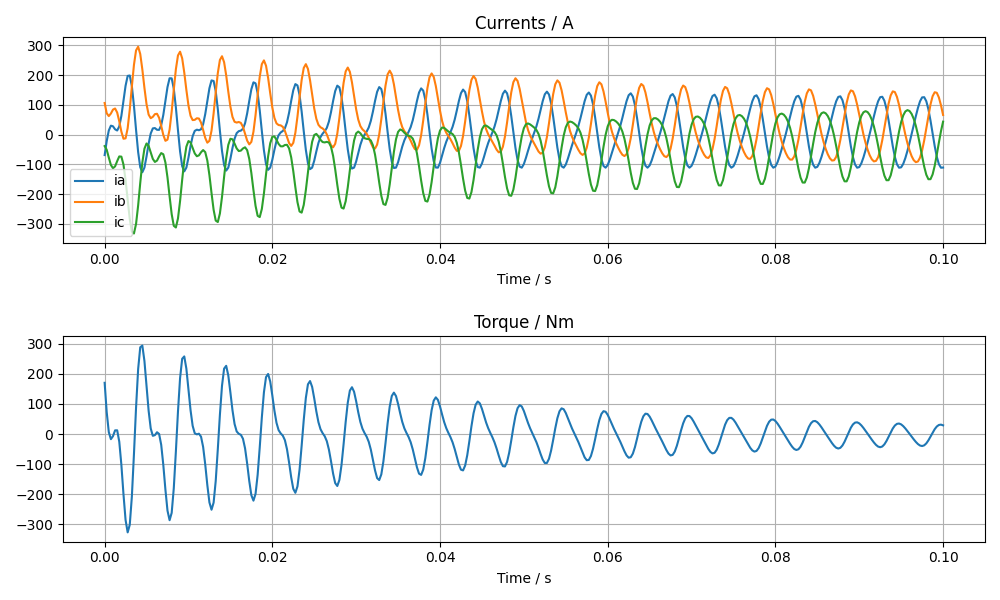
The short circuit calculation is executed subsequentially to a pm_sym_fast simulation if shortCircuit is set True. (version added 0.9.30). The results are included in scData dict of bch

Parameter	Description	Default	Unit
shortCircuit	run short circuit calc if True
l_end_winding	winding inductance	0	H
l_external	External inductance	0	H
sc_type	type of short circuit (3-phase)	3
simultime	Simulation time	0.1	s
initial	Initial condition 1: noload 2: load	2
allow_demagn	Allow Demagnetisation:1:yes; 0:no	0
sim_demagn	Simulate Demagnetisation:1:yes; 0:no	0

Example:

pmRelSim = dict(
   angl_i_up=-39.3,
   calculationMode="pm_sym_fast",
   wind_temp=60.0,
   magn_temp=60.0,
   current=76.43,
   period_frac=6,
   speed=50.0,
   shortCircuit=True,
   l_end_winding=0,
   l_external=0,
   sc_type=3,
   initial=2,
   allow_demagn=0,
   sim_demagn=1)

r = femag(machine,
       pmRelSim)

print('Torque [Nm] = {}'.format(r.machine['torque']))
print('''
  Short Circuit    Current         Torque
    Peak       iks {2:8.1f} A  tks {3:8.1f} Nm
    Stationary ikd {0:8.1f} A  tkd {1:8.1f} Nm

  peak winding currents {4}
'''.format(r.scData['ikd'],
           r.scData['tkd'],
           r.scData['iks'],
           r.scData['tks'],
           r.scData['peakWindingCurrents']))

fig, ax = plt.subplots()
femagtools.plot.transientsc(r)
plt.show()

Ld-Lq Identification (ld_lq_fast)

Parameter	Description	Default	Unit
speed	Speed		1/s
skew_angle	Skewing angle	0	deg
num_skew_steps	Number of skew steps	0
magn_temp	Magnet Temperature		°C
num_move_steps	Number of move steps
num_par_wdgs	Number of parallel windings	1
eval_force	Evaluate force	0
i1_max	Max. phase current		A (RMS)
beta_min	Min. Beta angle		deg
beta_max	Max. beta angle		deg
num_cur_steps	Number of current steps
num_beta_steps	Number of beta steps
period_frac	Rotate Fraction of Period	1

Example:

feapars = dict(
  num_move_steps=25,
  calculationMode="ld_lq_fast",
  magn_temp=60.0,
  i1_max=150.0,
  beta_max=0.0,
  beta_min=-60.0,
  num_cur_steps=3,
  num_beta_steps"=4,
  speed=50.0)

Psid-Psiq Identification (psd_psq_fast)

Parameter	Description	Default	Unit
speed	Speed		1/s
skew_angle	Skewing angle	0	deg
num_skew_steps	Number of skew steps	0
magn_temp	Magnet Temperature		°C
num_move_steps	Number of move steps
num_par_wdgs	Number of parallel windings	1
eval_force	Evaluate force	0
maxid	Max. Amplitude Id current		A
minid	Min. Amplitude Id current		A
maxiq	Max. Amplitude Iq current		A
miniq	Min. Amplitude Iq current		A
delta_id	Delta of Id current steps		A
delta_iq	Delta of Iq current steps		A
period_frac	Rotate Fraction of Period	1

Example:

feapars = dict(
  num_move_steps=25,
  calculationMode="psd_psq_fast",
  magn_temp=60.0,
  maxid=0.0,
  minid=-150.0,
  maxiq=150.0
  miniq=0.0,
  delta_id=50.0,
  delta_iq=50.0,
  speed=50.0)

PM/Rel Torque Calc (torq_calc)

Parameter	Description	Default	Unit
speed	Speed		1/s
skew_angle	Skewing angle	0	deg
num_skew_steps	Number of skew steps	0
magn_temp	Magnet Temperature		°C
wind_temp	Winding Temperature	20	°C
num_move_steps	Number of move steps	49
num_par_wdgs	Number of parallel windings	1
current	Phase current		A (RMS)
angl_i_up	Angle I vs. Up	0	deg

Example:

operatingConditions = dict(
  calculationMode="torq_calc",
  wind_temp=60.0,
  magn_temp=60.0,
  current=50.0,
  angl_i_up=0.0,
  speed=50.0)

FE-Simulation with existing model¶

FE calculations can be executed for existing models also. Since Femag Rel 8.3 there is no need to fully specify the machine model:

machine = "PM 270 L8"

workdir = os.path.join(
  os.path.expanduser('~'), 'femag')

femag = femagtools.Femag(workdir)

operatingConditions = dict(
  angl_i_up=-38.7,
  calculationMode="pm_sym_fast",
  magn_temp=60.0,
  num_move_steps=25,
  speed=50.0,
  wind_temp=60.0,
  current=108.0)

r = femag(machine,
          operatingConditions)

For older FEMAG versions the minimal data is:

machine = dict(
    name="PM 130 L4",
    lfe=0.1,
    poles=4,
    outer_diam=0.13,
    bore_diam=0.07,
    airgap=0.001,

    stator=dict(
        num_slots=12,
        num_slots_gen=3,
        mcvkey_yoke="dummy"
    )
)

Model Creation with DXF¶

The goal of the dxfsl modules is to create a complete FE model for rotating PM and Reluctance Machines on the basis of a DXF file with as little restrictions as possible. This has the consequence that symmetries, subregions, magnets, windings, boundary conditions need to be identified.

The procedure is as follows:

Read the DXF file and create a graph object with nodes and edges.
Identify the areas stator, rotor and airgap and their symmetry axis.
Add auxiliary lines if required by the meshing process.
Convert the graph object into FSL code including the identified subregions.

For monitoring and trouble-shooting purposes it is possible to create plots that display the intermediate results.

Example with a single dxf file motor.dxf:

machine = dict(
   name="Motor",
   lfe=0.001,

   dxffile=dict(
      name='motor.dxf'
   ),
   stator=dict(
      mcvkey_yoke='dummy',
      mcvkey_shaft="dummy"
   ),
   magnet=dict(
      mcvkey_yoke="dummy",
      mcvkey_shaft="dummy"
   ),
   ...

Note

The parameters poles, outer_diam, bore_diam and airgap as well as num_slots and num_slots_gen will be set automatically

Example with two separate dxf files for stator and rotor:

machine = dict(
   name="Motor",
   lfe=0.001,

   stator=dict(
       mcvkey_yoke='dummy',
       dxffile=dict(
           name='mystator.dxf',
           position='out',
           split=True
      )
   ),
   magnet=dict(
       mcvkey_yoke="dummy",
       mcvkey_shaft="dummy",
       dxffile=dict(
           name='myrotor.dxf',
           position='in',
           split=True
       )
   ),
   ...

Table of Contents

Previous topic

Next topic

This Page

Models¶

Machine¶

Stator¶

Stator Slots¶

User defined Stator Slots with FSL¶

User defined Slots with DXF¶

Windings¶

Magnet¶

Rotor Slots¶

User defined Magnet Slots with FSL¶

User defined Slots with DXF¶

Magnetizing Curve¶

Magnet Material¶

User Specified Magnet Geometries¶

FE-Simulation¶

FE-Simulation with existing model¶

Model Creation with DXF¶

Name	Parameter	Unit
perimrad	Radius of perimeter	m
vbendrad	Bending radius vertical	m
endheight	End winding height	m
m.wiredia	Wire diameter	m